-Boyu Zhu

Proj1: High Dynamic Range

Background

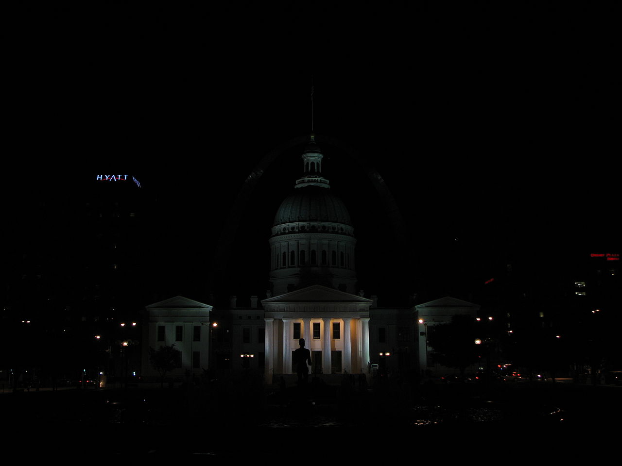
Modern cameras are unable to capture the full dynamic range of commonly encountered real-world scenes. In some scenes, even the best possible photograph will be partially under or over-exposed. Researchers and photographers commonly get around this limitation by combining information from multiple exposures of the same scene.

Radiance map construction

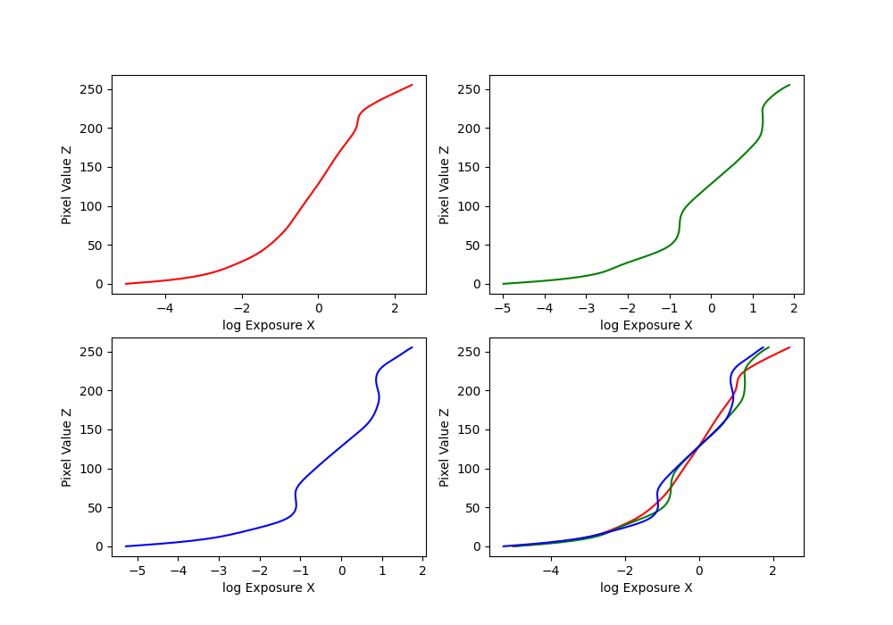
We want to recovering a radiance map from a collection of images. So we want to find the funcion g and therefore to get the log radiance values for each pixel. Based on the equation below, we can
use the function g and the known exposure durations in the above equation to generate an average radiance image from the set of input images. Again use a weighted average that gives more weight to pixels in the middle of the captured image range.

First, I use the arch image

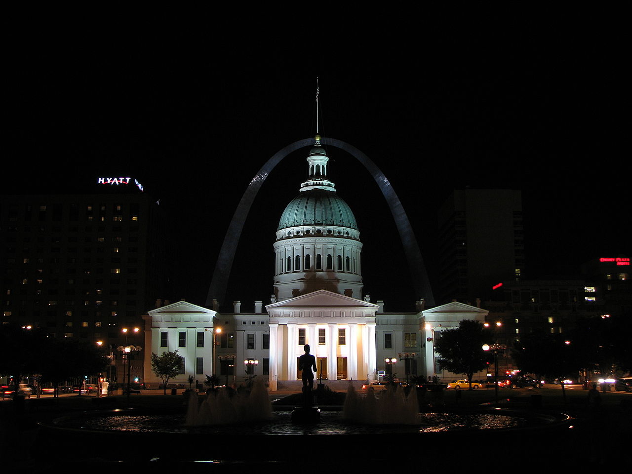
Here is the functions approximate for the arch image

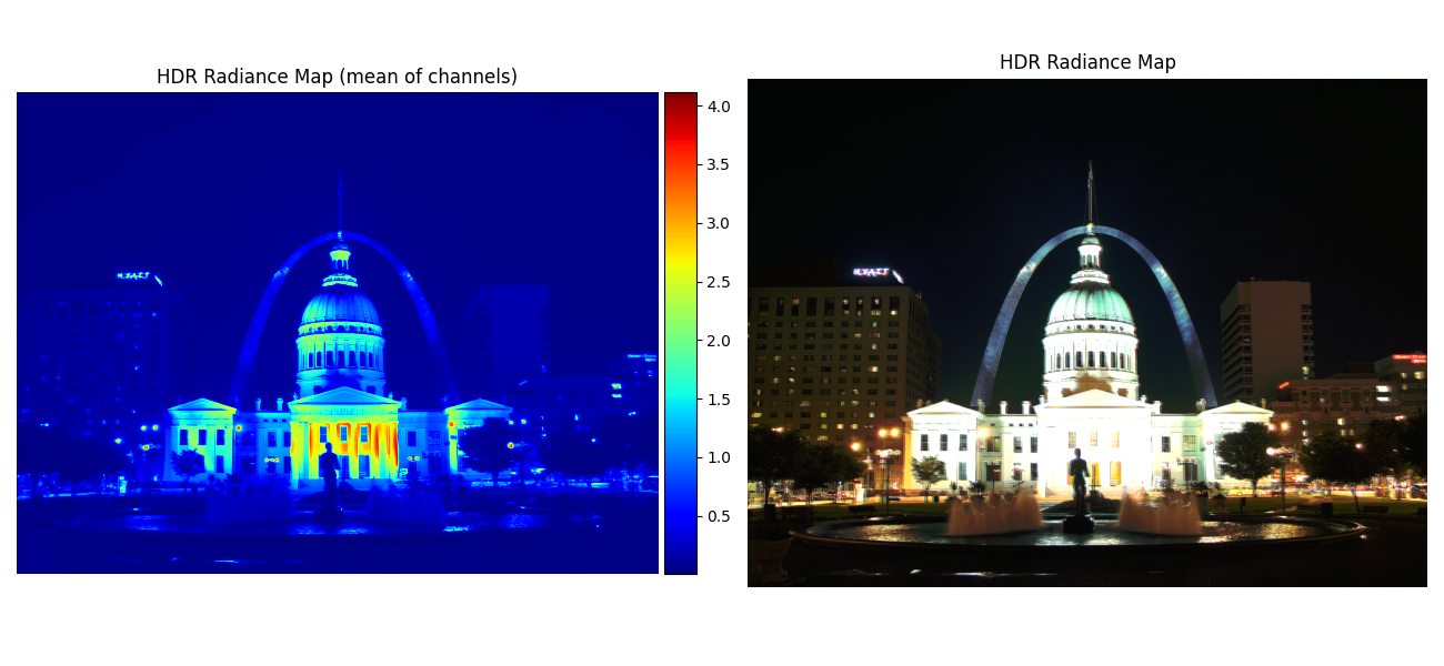
The radiance map of the image

Tone mapping

However, only getting the radiance map is far from enough. We apply tone mapping to stretch the intensity values in the resulting image to fill the [0 255] range for maximum contrast.

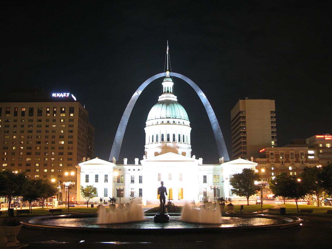
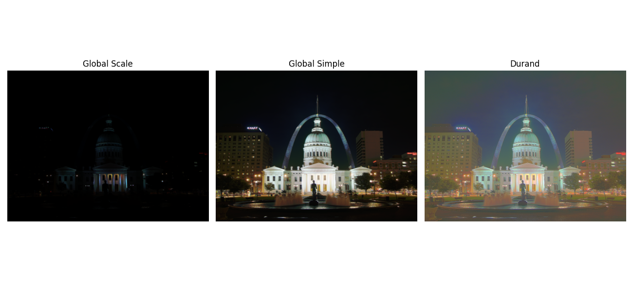
In this part, we apply three kinds of tone mapping techniques.

• Global scaling: clip the data between 0 and 1

• Global simple: $E'_i = \frac{E_i}{1+E_i}$, based on the equation, to map the pixel to 0 and 1

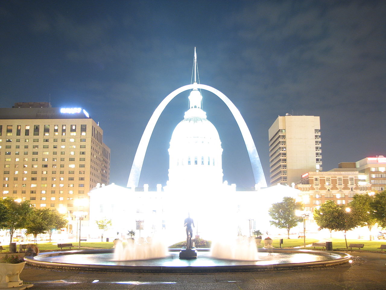
• Durand: (the following steps are from project spec)

1 Your input is linear RGB values of radiance.

2 Compute the intensity (I) using a luminance function (such as MATLAB's rgb2gray)

3 Compute the chrominance channels: (R/I, G/I, B/I)

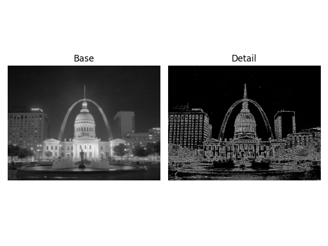
4 Compute the log intensity: L = log2(I)

5 Filter that with a bilateral filter: B = bf(L)

6 Compute the detail layer: D = L - B

7 Apply an offset and a scale to the base: B' = (B - o) * s

8 Reconstruct the log intensity: O = 2^(B' + D)

9 Put back the colors: R',G',B' = O * (R/I, G/I, B/I)

10 Apply gamma compression. Without gamma compression the result will look too dark. Values around 0.5 should look fine (e.g. result.^0.5)

In this part, I used the bilateral filter to get the Detail Layer and Base Layer. (The Detail Layer is binarized for display, threshold = 0.1)

And below are the results for all images:

Global Simple

Durand

The results are incredible, and are much better compared to the original result. From eyed debugging, we cannot say that the Durand method is completely better than the Global Simple method, because there are some scenes where the Durand method does not seem to have an advantage. My conclusion is that when the span of the maximum and minimum values of the radiation diagram is relatively small, the Global Simple method is better. However, if the span is very large, such as when the contrast between bright and dark parts is large, for instance outdoors images, the Durand method performs better.

Bells and Whistle: Try the algorithm on your own photos!

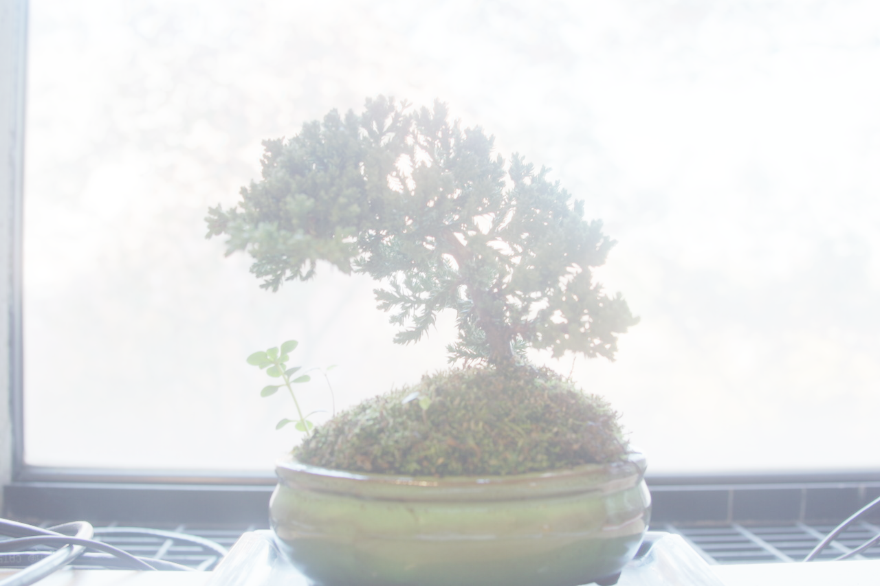
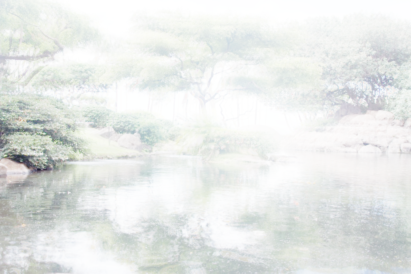
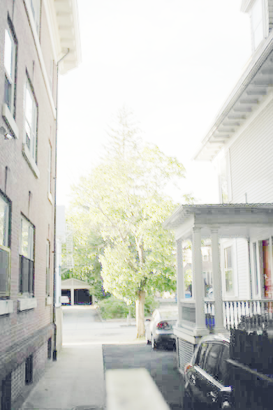
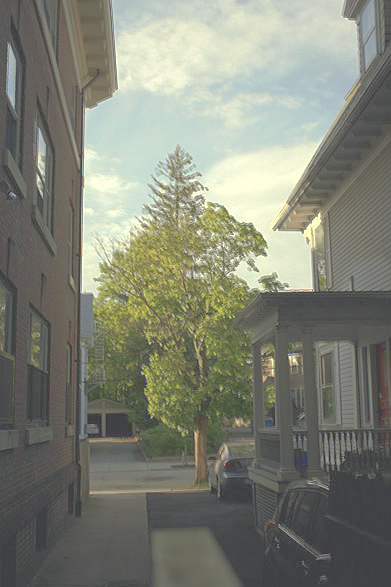
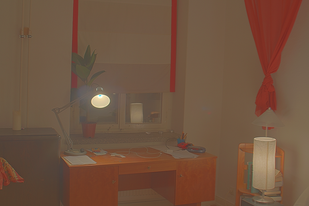
I took the photos of the corridor of my apartment, and inside the building, it was rather dark, while it is very bright outside the building.

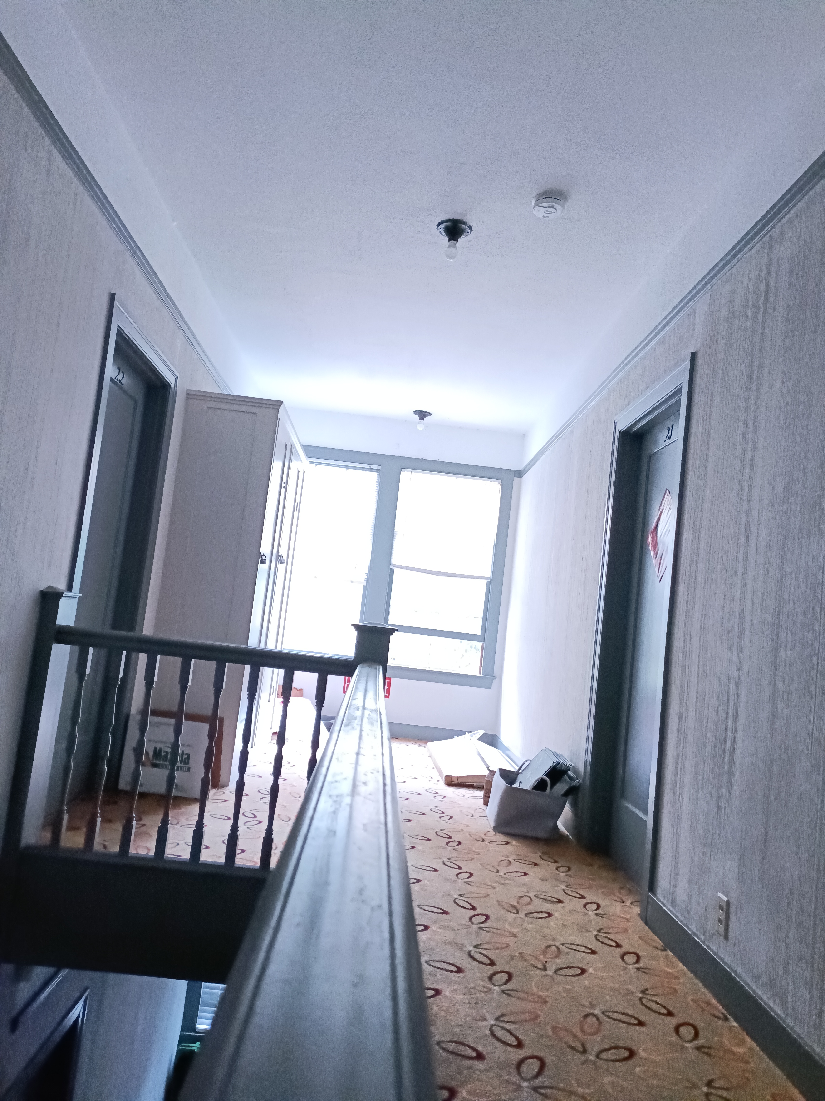
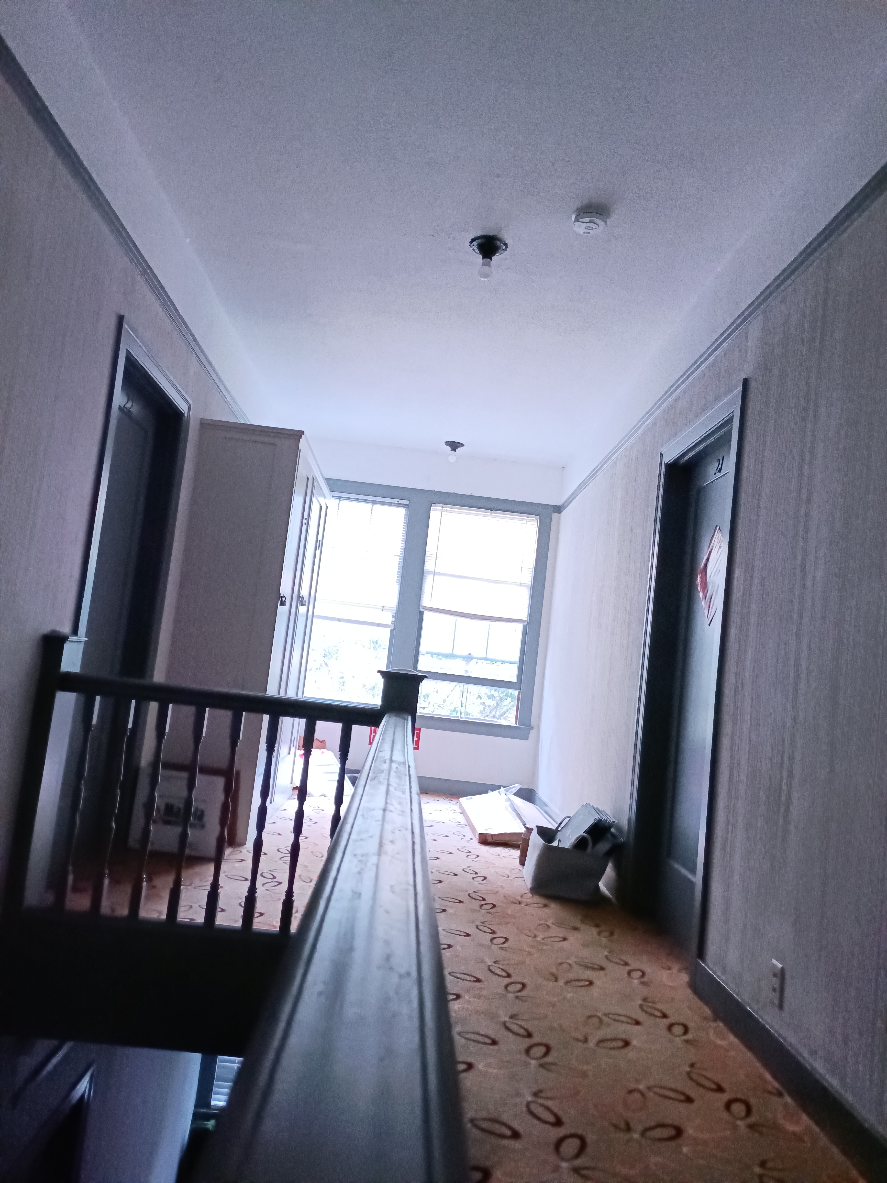
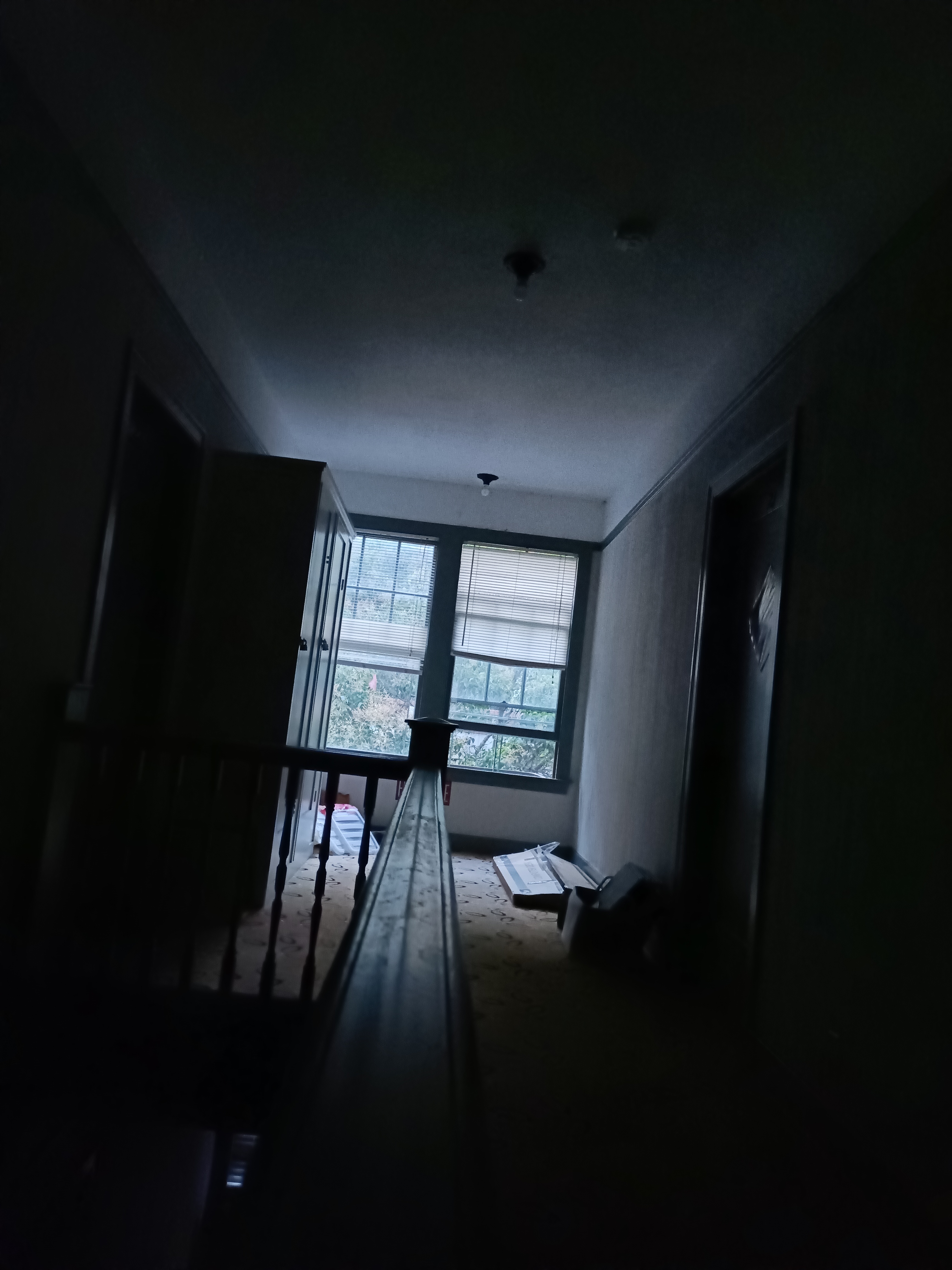
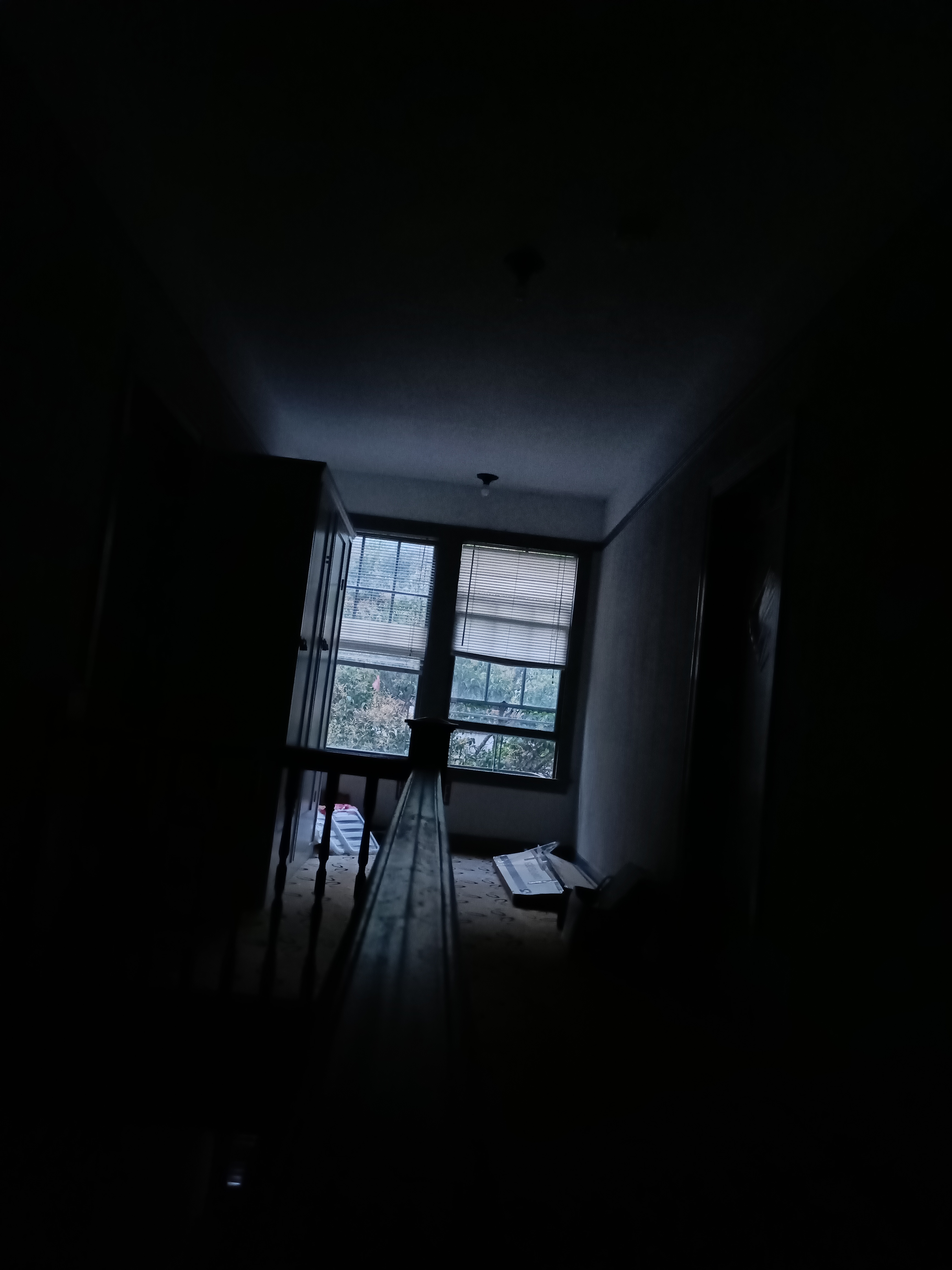
I try the algorithm on the images. And the result is amazing

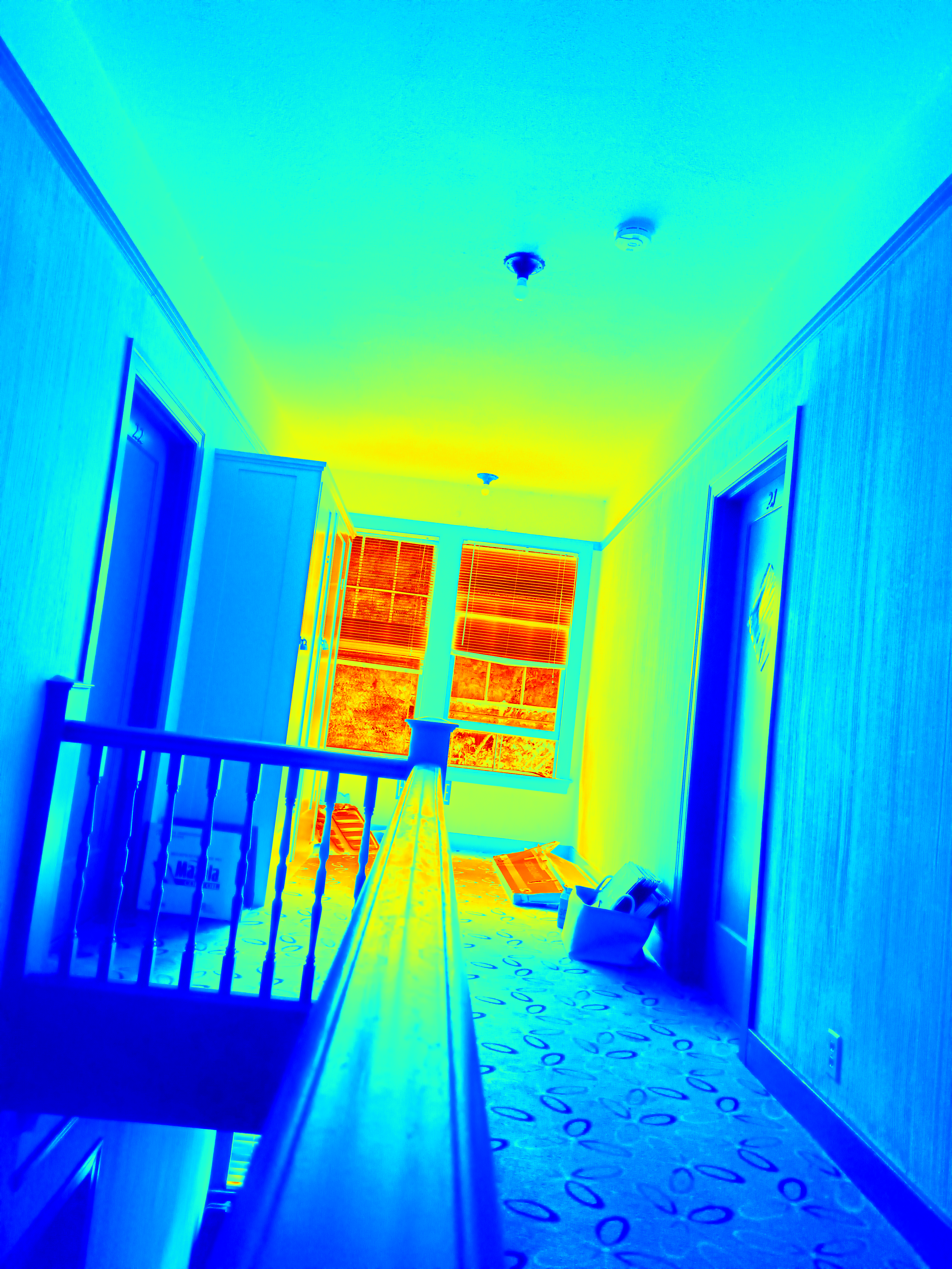
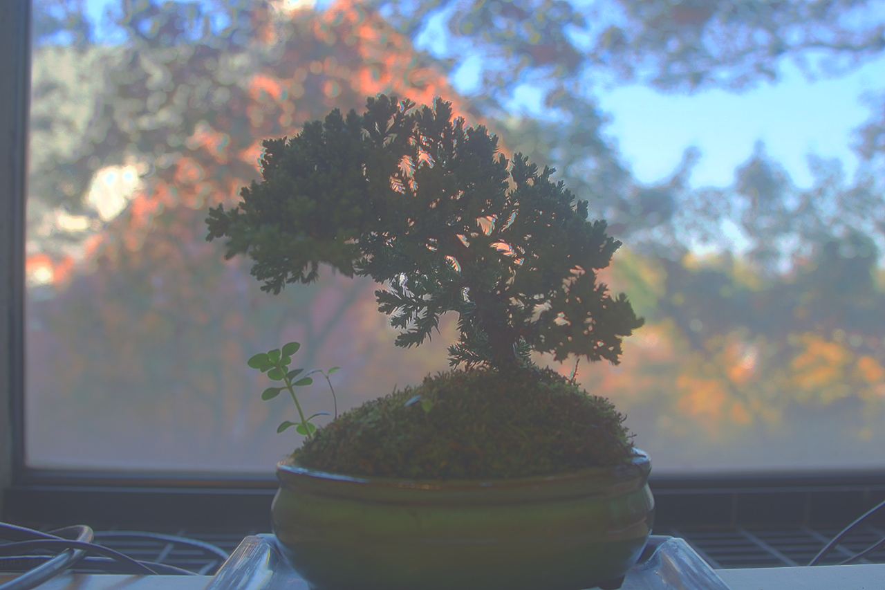
heatmap

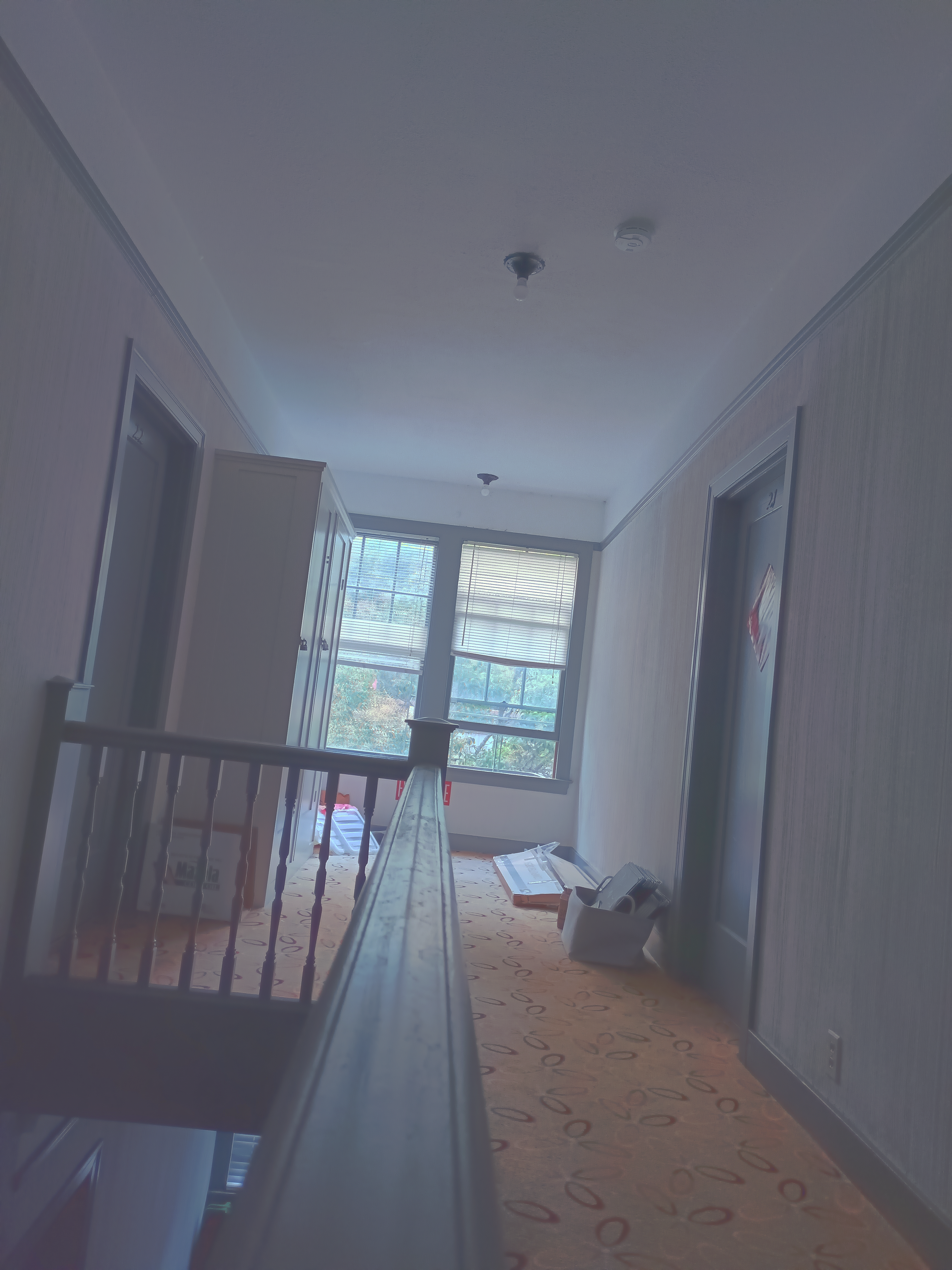
durand

The radiance map show the strength of each pixel, which aigns with the intuition, and the durand algorithm capture the bright part and the dark part at the same time.

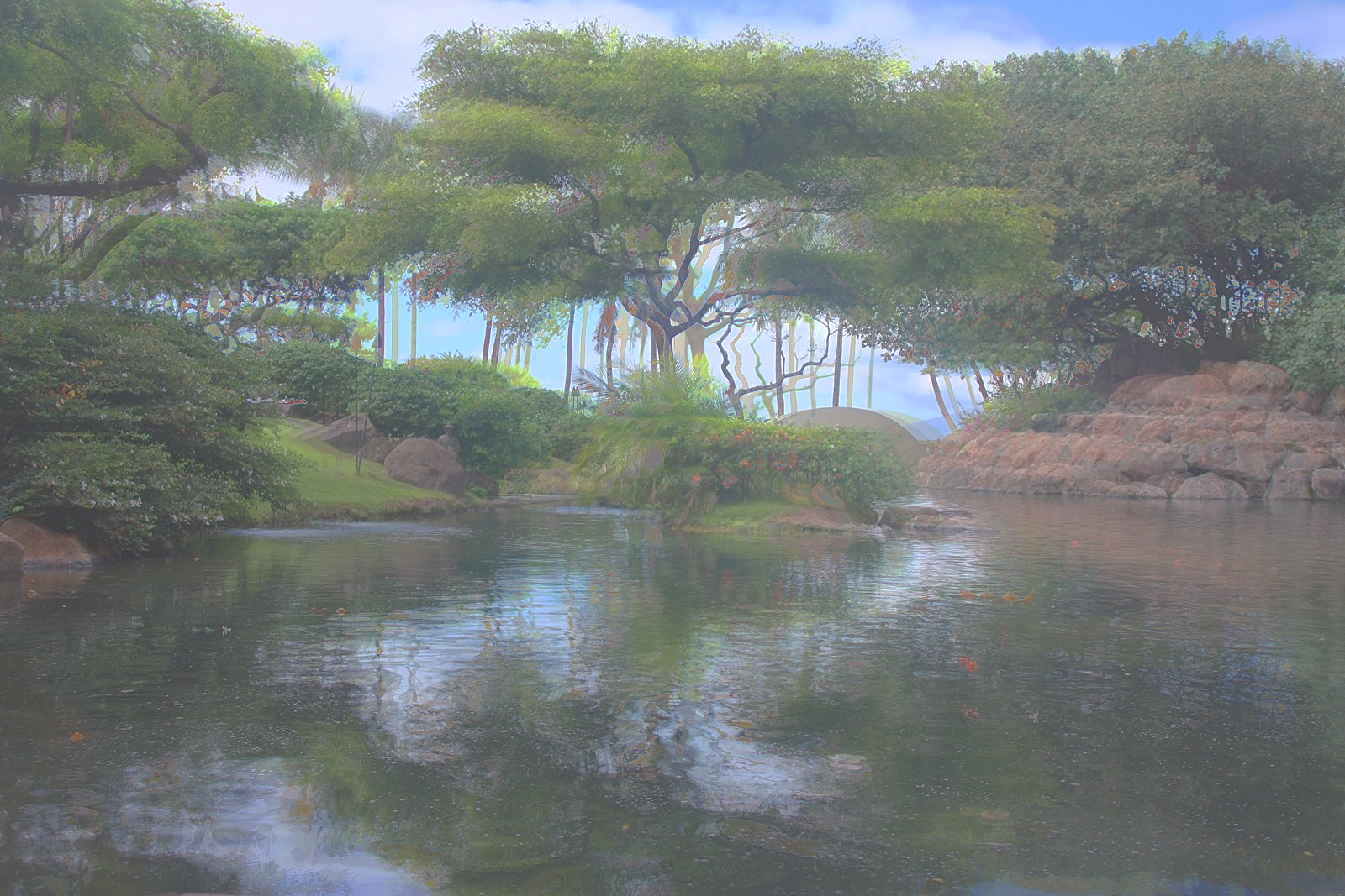
Bells and Whistle: automatic alignment

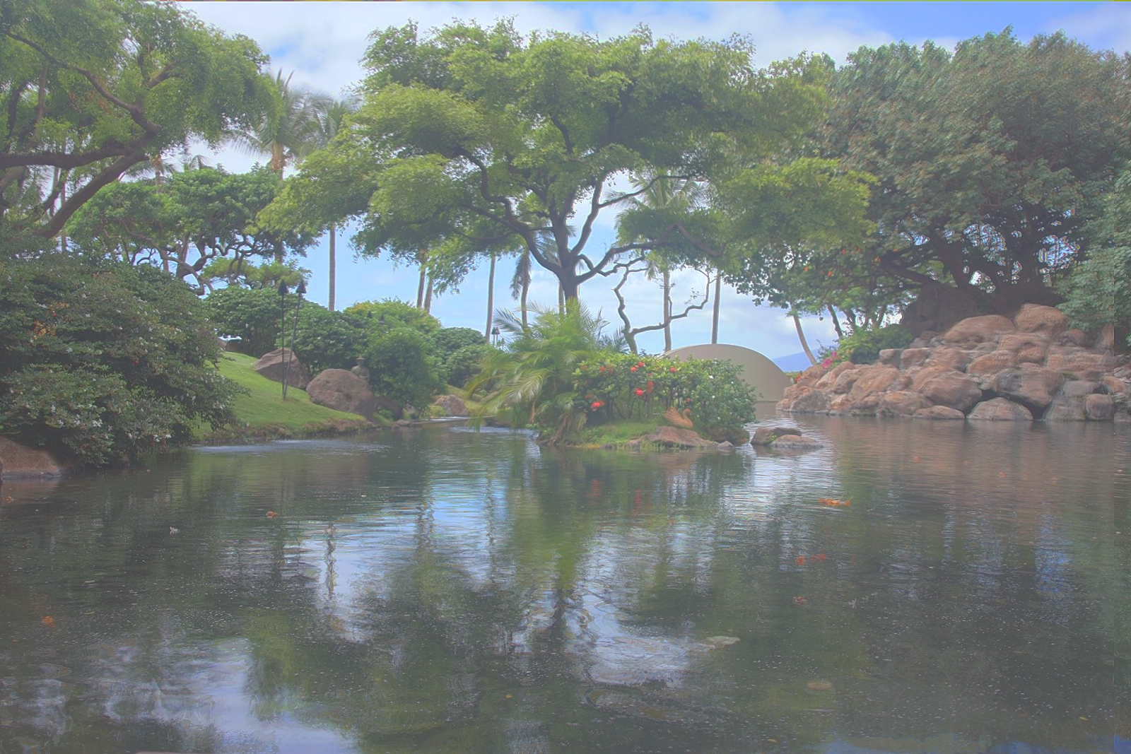
We can see that for image for example garden, the images didn’t align very well, so it is important to apply alignment before the hdr mapping process begins.

before alignment

For this aim, I use the cv2.createAlignMTB() method to automatically align the image before the process begins, and we can witness a large improvement in the final hdr image quality.

after alignment

The improvement is obvious.

Proj2: Lightfield Camera: Depth Refocusing and Aperture Adjustment with Light Field Data

In this part, we want to reproduce depth refocusing and Aperture Adjustment using real lightfield data.

For datast, we use The Stanford Light Field Archive , which has multiple images taken over a regularly spaced grid.

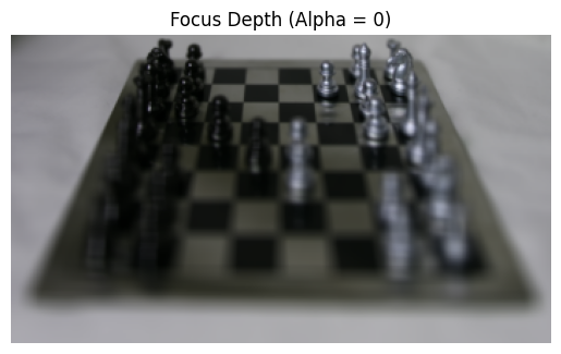
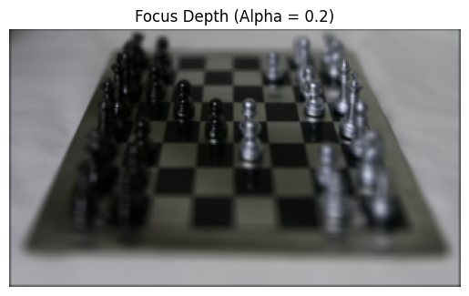
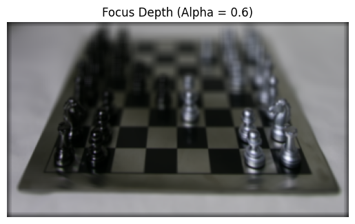
1) Depth Refocusing

First, we can simply average all the images together and see what will happen.

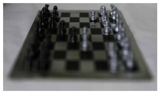
We can see that the photo is focused at far away. The objects which are far away from the camera do not vary their position significantly when the camera moves around while keeping the optical axis direction unchanged. However, those points will change greatly. That’s why the picture look sharp in the far end while it is blurry in the near place.

Therefore we can shifting the images to a centralized reference multiplied by a factor α, along with averaging, allows one to focus on object at different depths.

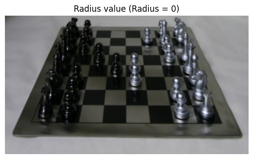
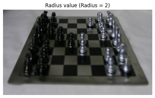
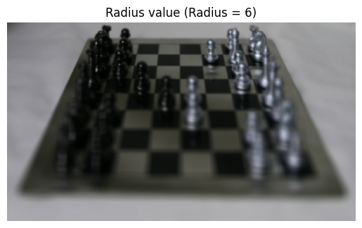
2) Aperture Adjustment

For the second part, we want to explore how to adjust the Aperture with the dataset.

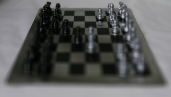
What we do is we first select the picture at the center of the scene, and then by changing the radius, we choose those pictures around the center within the radius.

3) Summary

This project is amazing! I like taking photos, but I always struggle with choosing focus and aperture, I never imagined that I could change these automatically through multiple photos, this is very interesting