Project 4: Stitching Photo Mosaics

-Boyu Zhu

PartA IMAGE WARPING and MOSAICING

1 Shoot and digitize pictures

Followed the requirements and recommendations, I shooted three sets of photos. Each set is chosen with some intention.

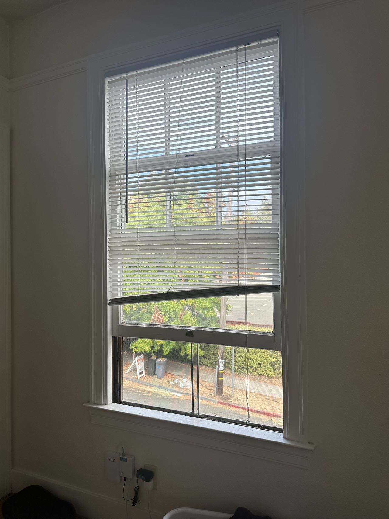
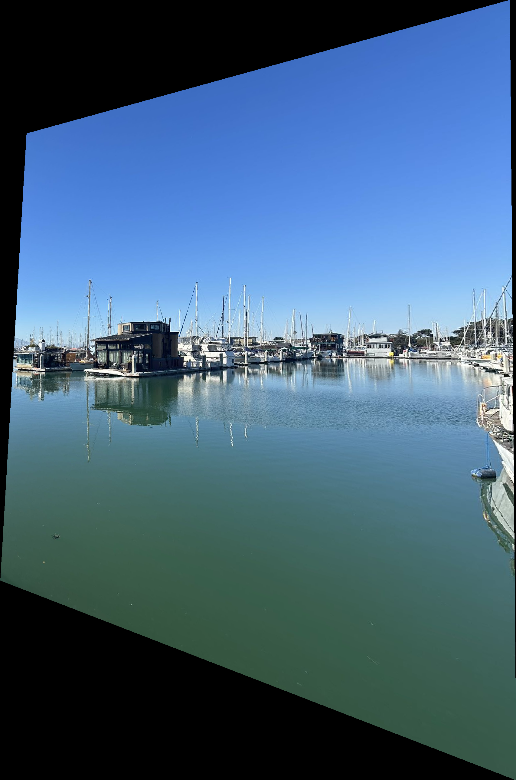
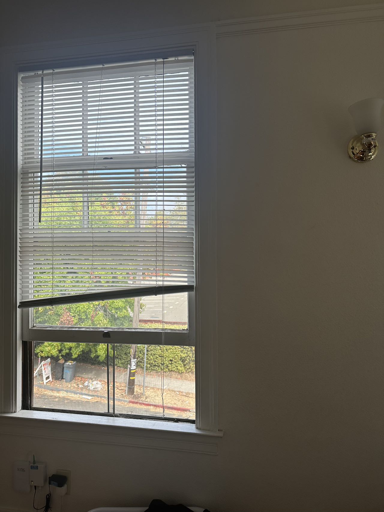
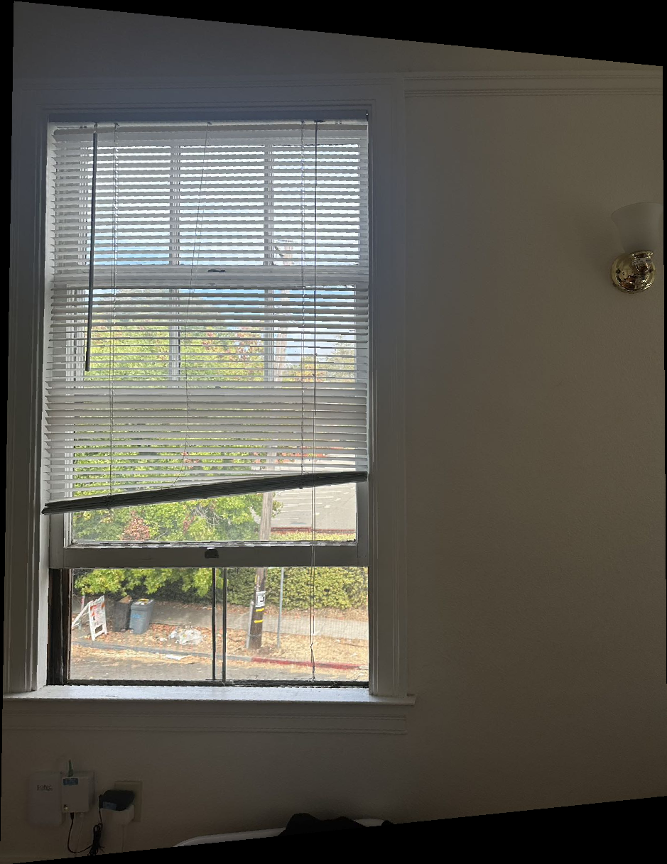
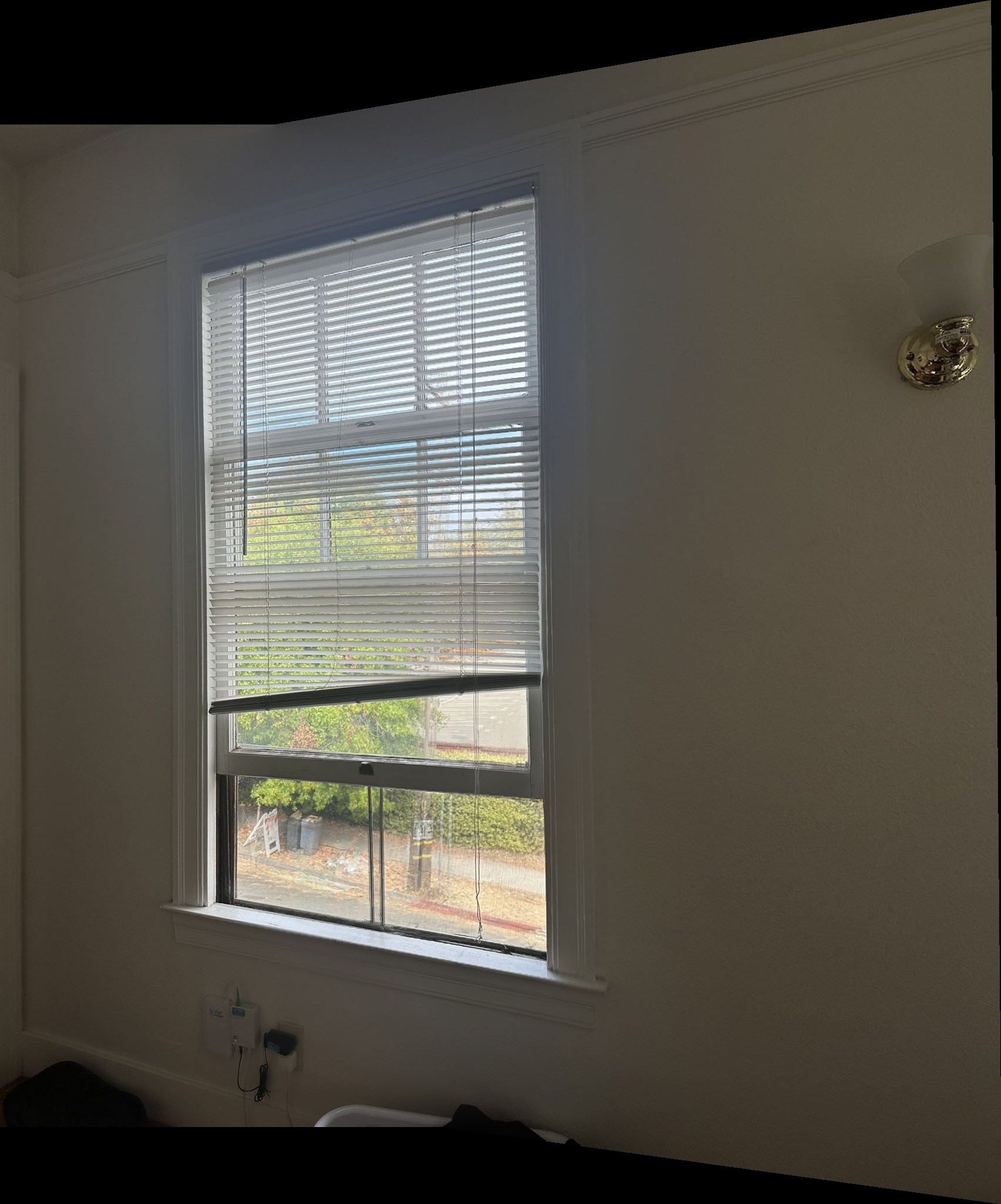
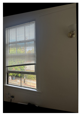
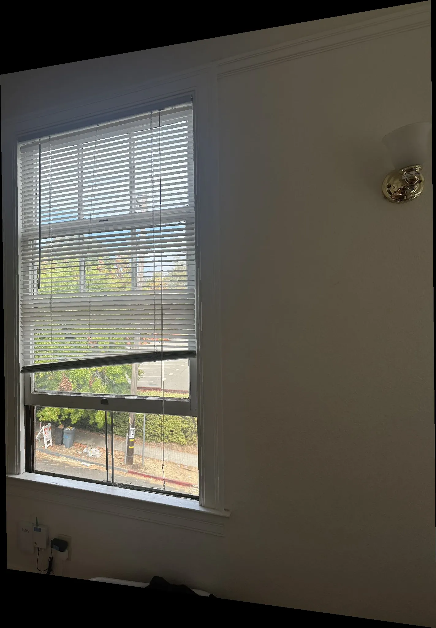
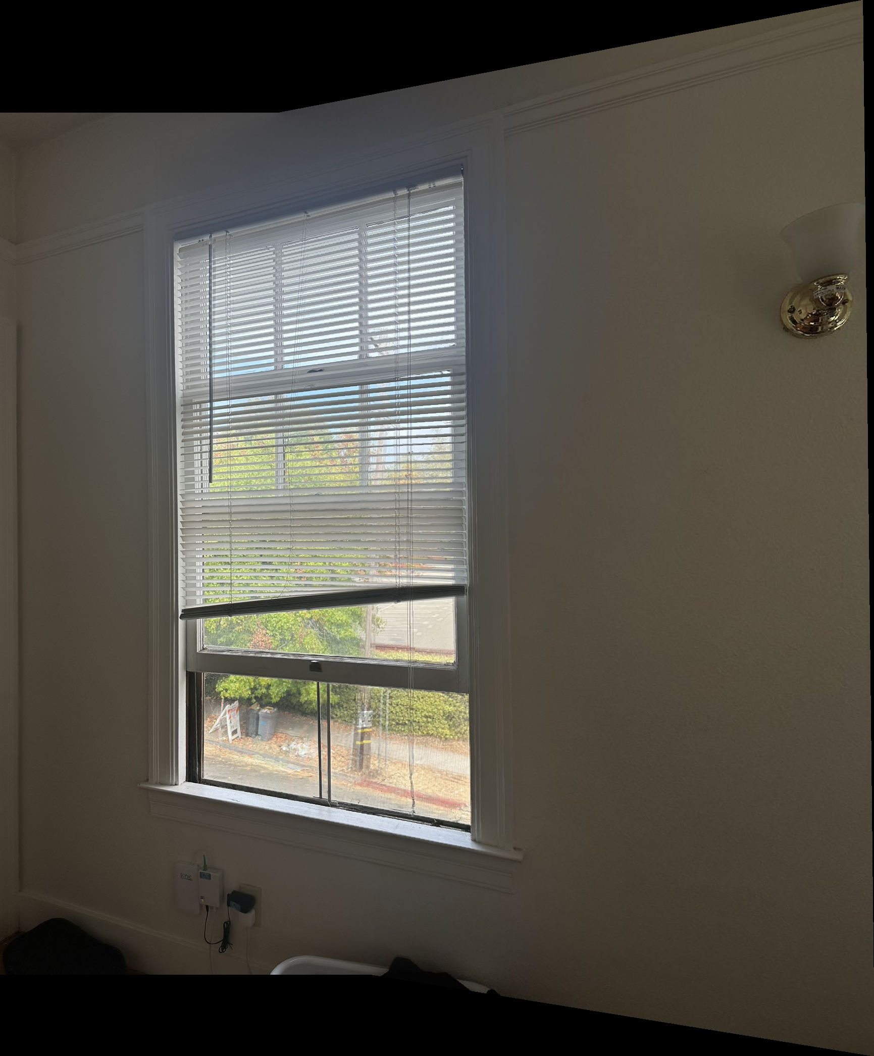
level 1: our apartment window and the beautiful view

Althogh from the same spot, the shape of the apartment window seem to form different shapes through the rotation the the camera, I tried to test whether this can be aligned perfectly.

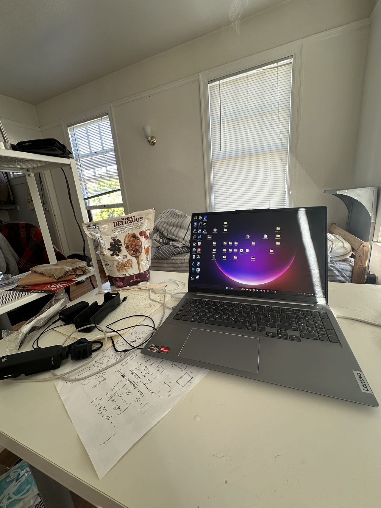
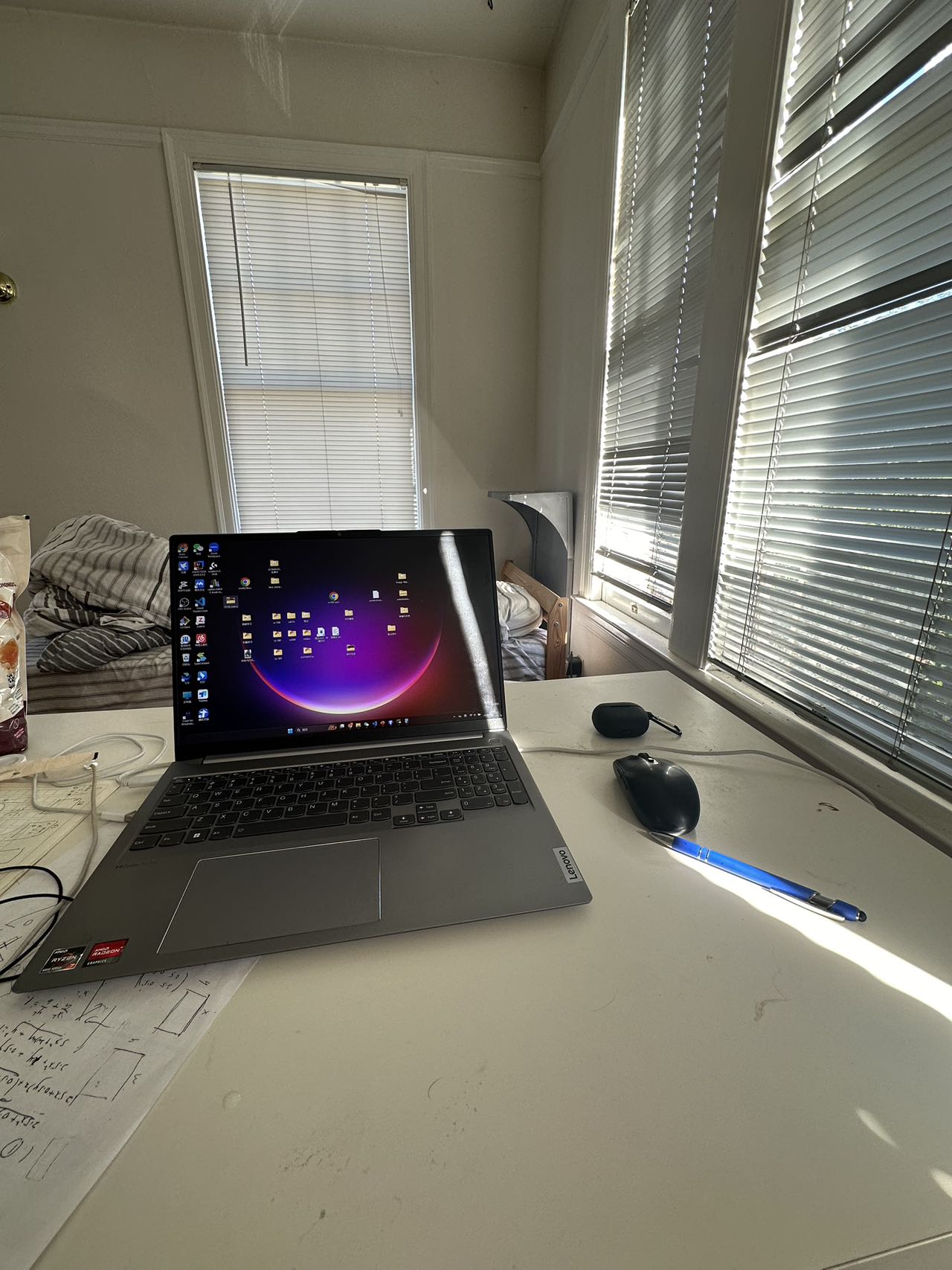
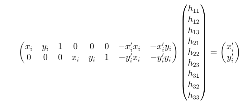
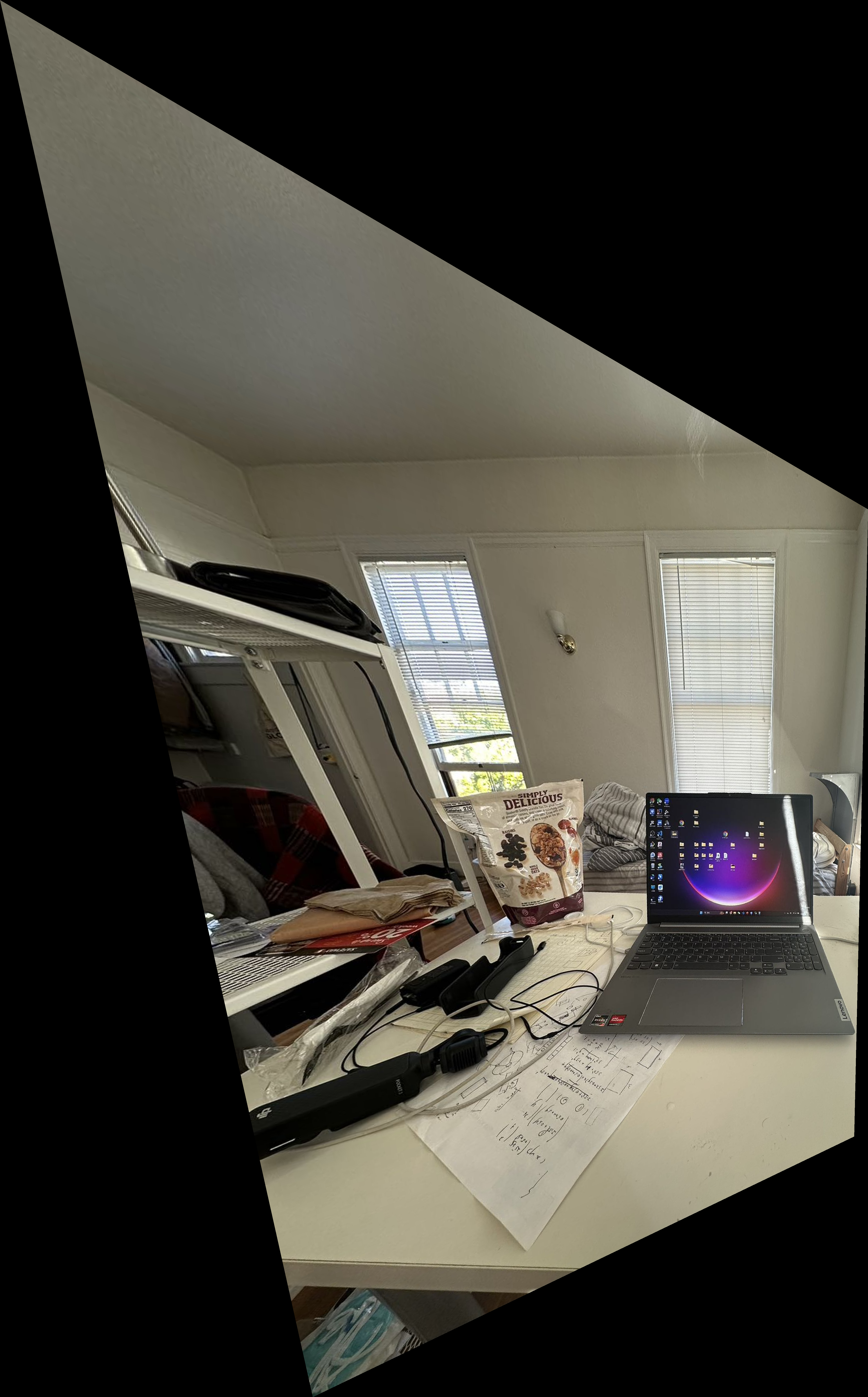
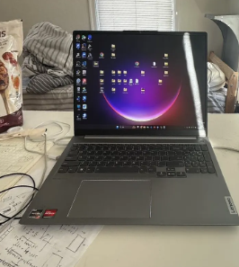
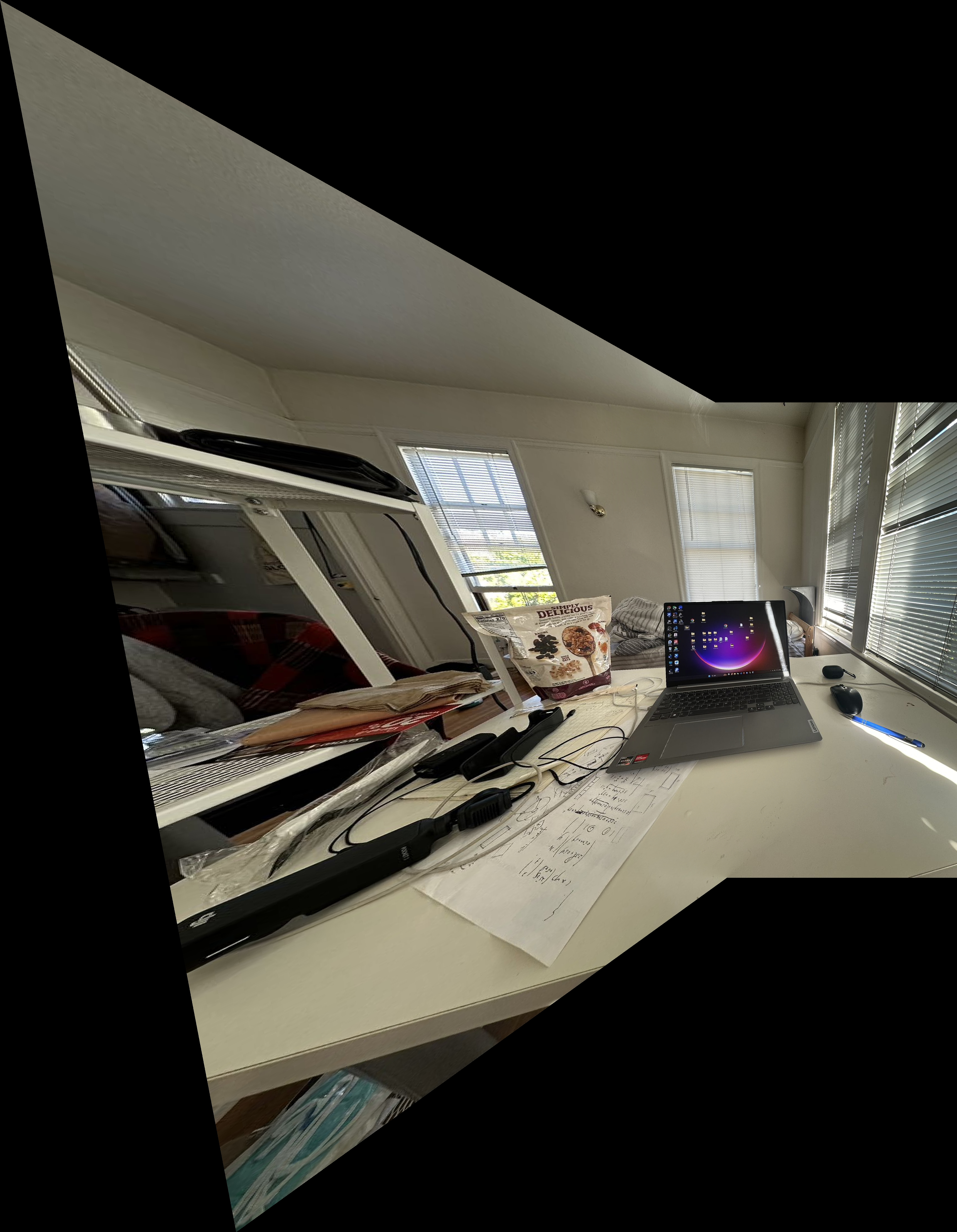
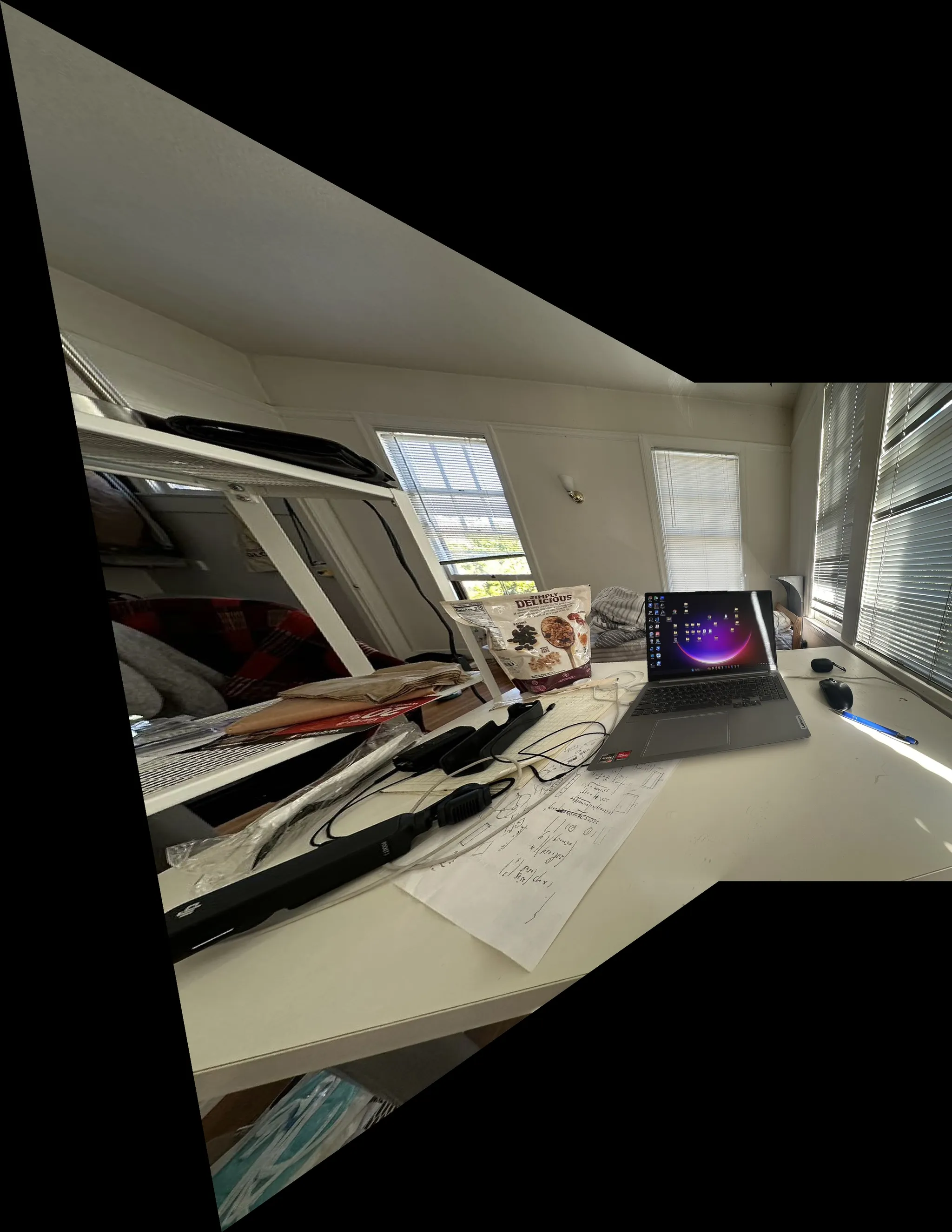
level 2: my table with laptop on it

There are a lot of small things on the desk and shelves, trying to see if this alignment is still possible.

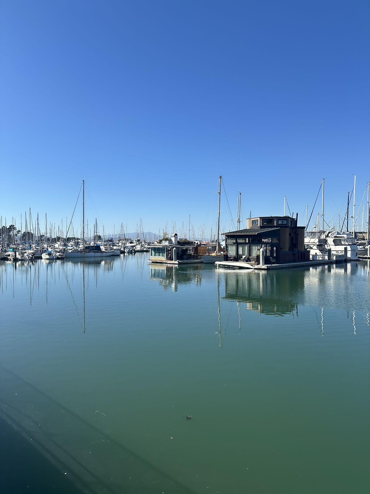
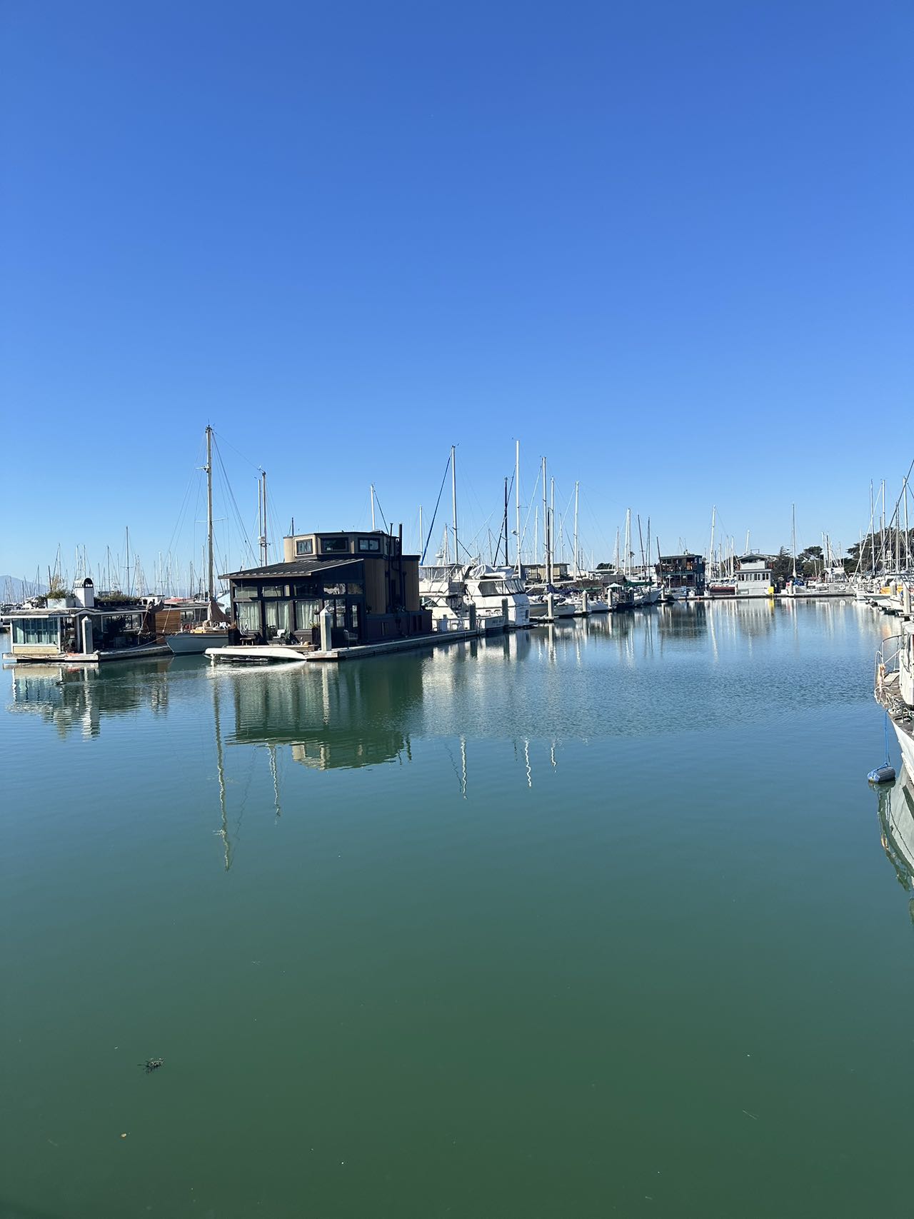
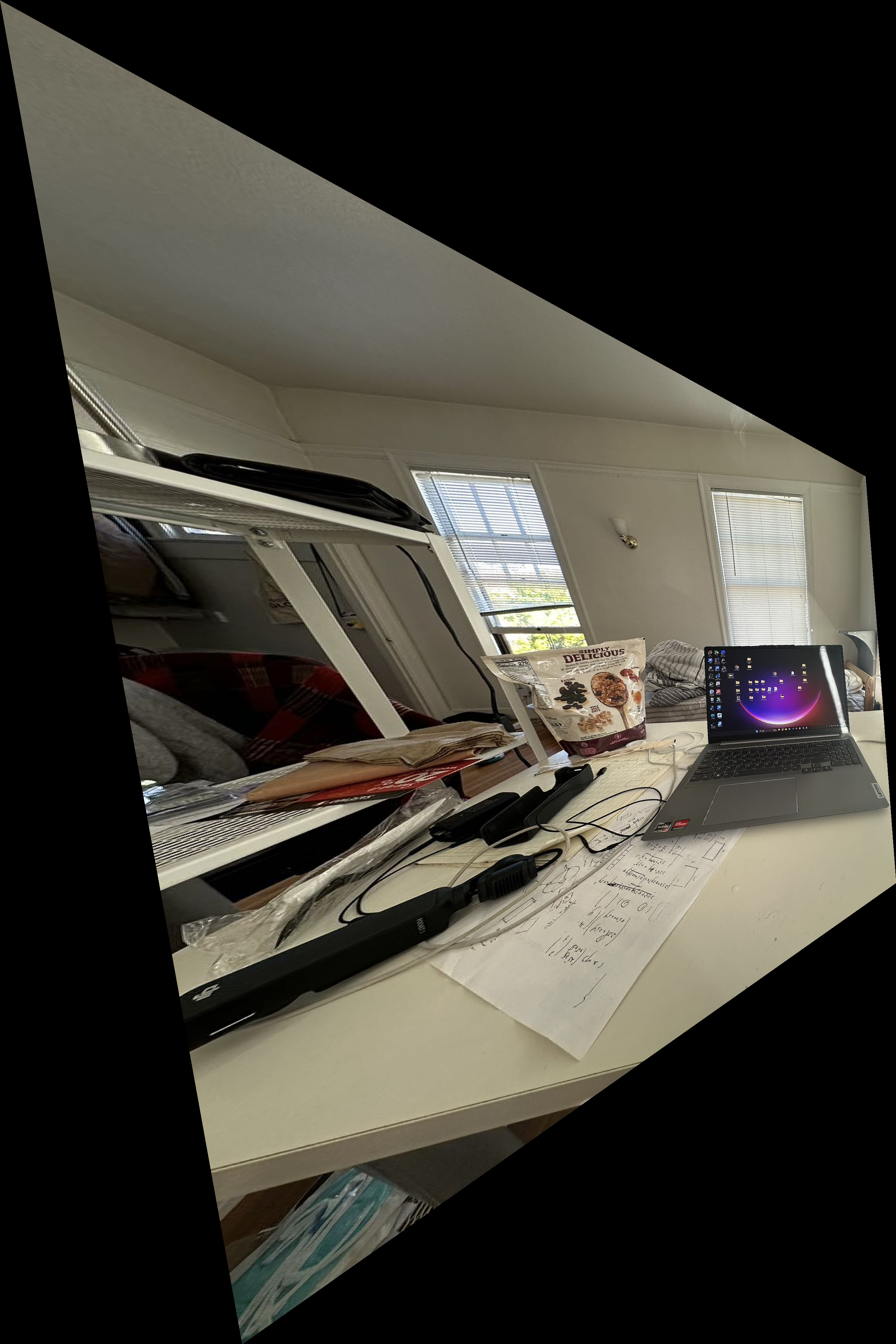
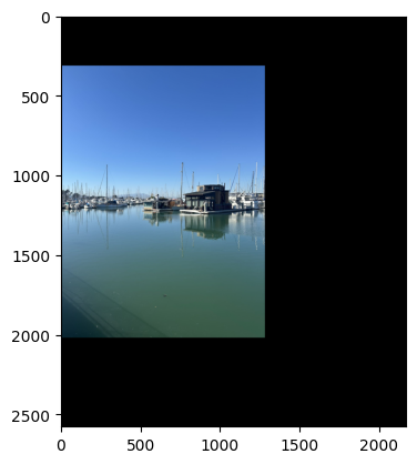
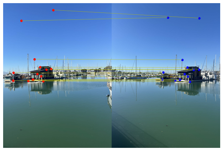
level3: Berkeley marina

There’re a jumble of boats and masts at Berkeley marina, it is a picture full of details.

And after shooting these images, I manually defined the correspondences of each two images.

Recover Homographies

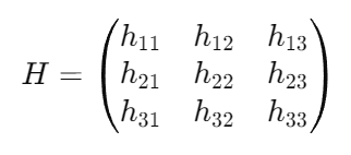
Our goal is to find a homography matrix to perform the transformation. The Homography matrix can be shown as: where

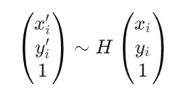
And the transformation can be represented as:

to compute the H matrix, we use the following linear equation

By including more than 4 correspondences, we’re now solving an overconstrained system using least squares.

Warp the Images

Now that we have the homography matrix, we can perform image warping.

However it’s kind of hard to do debuggin simply from eyes, therefore we can now perform “rectification” on the image.

Image Rectification

before

after

before

after

zoom in

Blend the images into a mosaic

For every set of pictures, I applied the same procedure, I warped both of the picture to the final canvas.

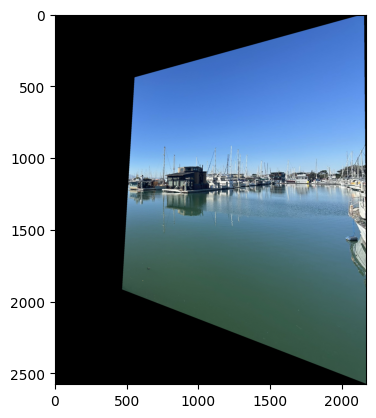
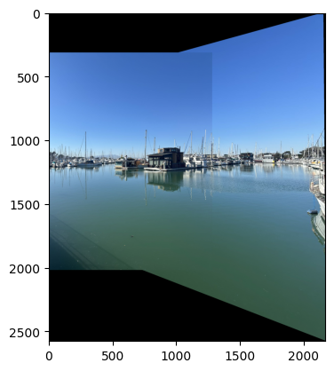
direct blended output

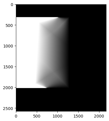
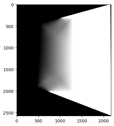
However, directly blending two images will cause strong edge artifacts, therefore I further explore ways to smoothly combine two images.

I employed a method using weighted blending and distance transform. In regions where only one of the images contains pixels, the weight for that image is set to 1. In the overlapping areas, a weighted sum determines the blending of the two images. The degree of blending is decided by the weighted sum of the distances from the pixel to the non-overlapping areas of both images.

And results are shown below.

PartB Automatic Correspondence Detection

Corner Detection

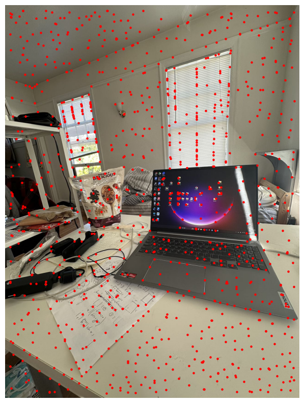
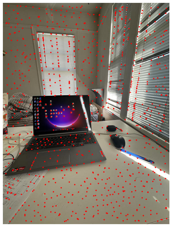
For the first part, we should first detct the potential feature points which can be used for for later alignment. We use Harris corner detection technique to detect the corner point in the picture. Using the sample code given in the spec, we can get the coordinations and strength of the corner points in the picture.

original image

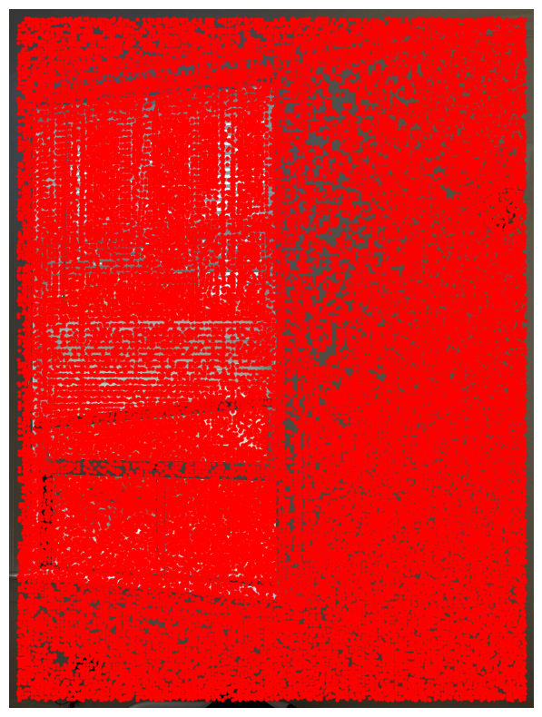
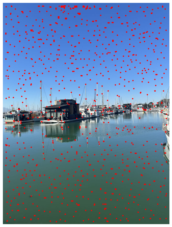
corner points

We can clearly see from the picture that the interest points is way too dense to be useful for the image feature matching.

Adaptive Non-maximal Suppression (ANMS)

To futher select interest points, I implements the non-maximal suppression technique described in the paper Multi-Image Matching using Multi-Scale Oriented Patches. The goal is to select feature points which are evenly distributed in the entire image and at the same time reduce the number of possible interest points. Specically, it determines the minimum suppression radius r by

$r_i = \min_{j} \left| x_i - x_j \right|, \quad \text{s.t. } f(x_i) < \text{crobust} f(x_j), \quad x_j \in I$

and then pick the largest n points to be our new interest points.

original image

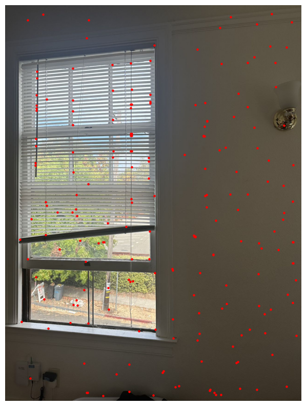
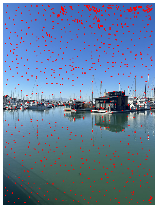
image after ANMS

We now can see that the interest points are much fewer now and they are evenly distributed over the picture.

Feature Descriptor Extraction

In this part, we can now extract the surrounding patch of the interest points. Each patch is axis-aligned and size of 40 * 40. Then we downsample it into 8 * 8 and apply normalizetion into that the mean is 0 and the standard deviation is 1.

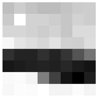
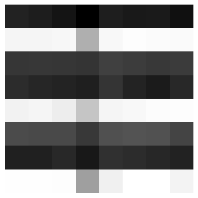
The descriptor now looks like this.

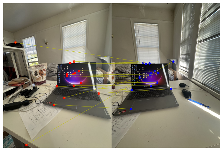
Feature Matching

In the feature matching part, we want to identify correspondences in the two pictures. And in this part, I use the Lowe’s trick to ensure that the pattern are actually ‘real’ correspondences.

the Lowe’s trick is that besides calculating the closest match, we also take the second closest match into considesation. If this ratio $ratio=\frac{d1}{d2}$ is below a certain threshold, the match is considered good. This can improve matching accuracy.

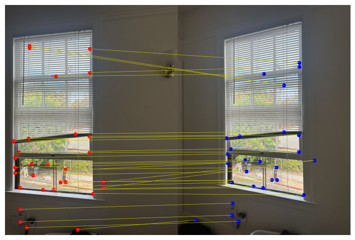
Random sample consensus RANSAC

Although we use Lowe’s trick to improve matching accuracy, however there’re still likely to have wrong matchings (can be seen in the picture above). Therefore, we use RANSAC to improve the robustness of the homography we compute.

The step are as follows: in every loop, we randomly choose four pairs of features, and then compute the homography, then we calculate the number of inliers, inliners are defined as $\text{dist}(\pi', H \pi) < \varepsilon$and we keep the Keep largest set of inliers, and at the end, we re-compute least-squares H estimate on all of the inliers.

After we get the homography, the following steps are similar to the first part.

warped image using the homography computed by RANSAC

part a warped result

part b warped result

and it is similar to the warped result in part a, which correspondences were manually chosen.

final result

result in part a

I can hardly tell the difference, all I can say is that the angle of the black edge on the far right of the picture is a little different

More Results

desktop

final result

result in part a

dock

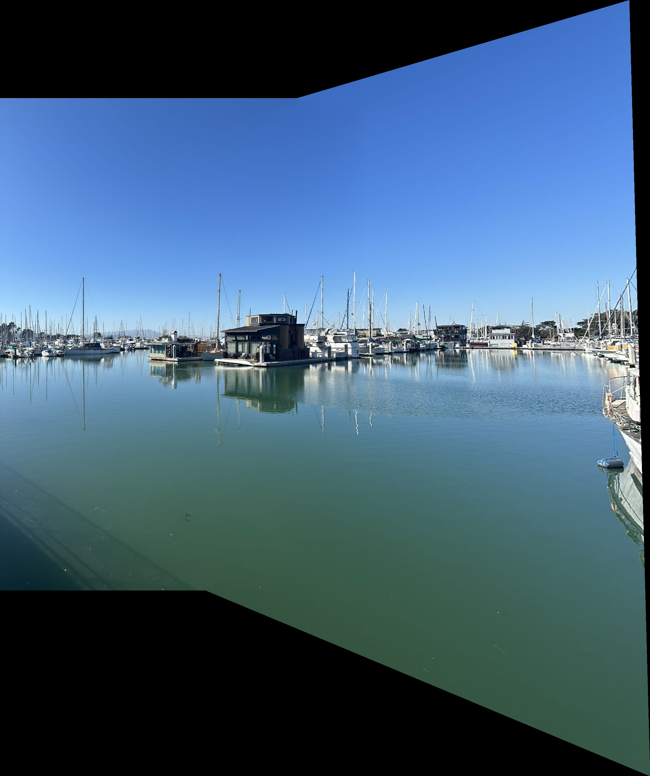
final result

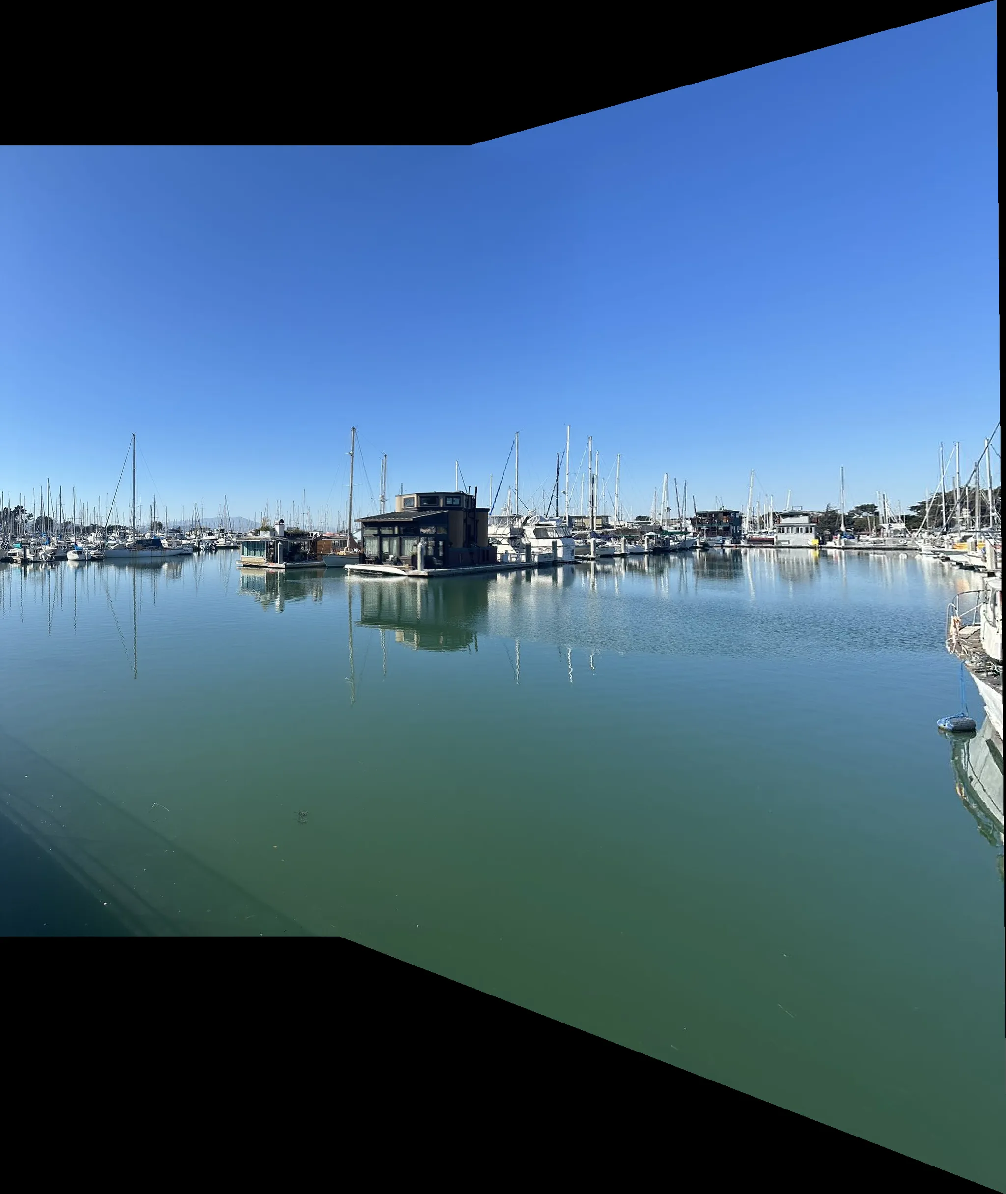
result in part a

I think these two examples show that the effect of this automatic program is completely comparable to the effect of carefully selecting a lot of corresponding points in part a.

What have you learned?

I think this project is very cool. The most impressive part is that now we can confidently give the task to computer to stitch the images, even with this basic approach, automatic stitching achieve impressive results, I can hardly tell the differences between the automatic version with the the manual version. So the machine has reached this level in this part, and I believe it can do much more cool things now and in future.